Regression problem (Linear reg. & K-nearest-neighbor)

Brief

In this article, we look at a regression problem, which falls into supervised statistical learning. I will discuss two main approaches: parametric and non-parametric approaches. Finally, we will compare the two.

Regression Problem

A regression problem falls under supervised statistical learning and assumes a quantitative dependent variable. For instance, temperature, sales, or the velocity of molecules.

Hence, in the equation:

\[Y = f(X) + \epsilon\]

the dependent variable $Y$ is quantitative. There are also independent variables $X$, a statistical model $f(X)$, and $\epsilon$, which is an irreducible error. There are two main approaches to this problem and statistical learning in general.

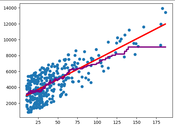
Figure 1: Simple linear regression in red and k-nearest-neighbor in purple.

Parametric Approach

Parametric approaches assume an explicit form of $f(X)$. For instance, $f(X) = \beta_0 + \beta_1 X + \beta_2 X^2$. Usually, coefficients $\beta_0, \;\beta_1, \;\beta_2$ have to be estimated from the data.

The advantage of the parametric approach is that it is usually straightforward to interpret the coefficients of the model. Furthermore, there is an intuitive sense of the relationship between predictors and dependent variables: linear, quadratic, etc. However, the disadvantage is that these models are quite inflexible. For instance, a linear model would perform poorly with data suited for a quadratic model.

Simple Linear Regression

For simple linear regression, assume that there is one independent and one dependent variable. In particular, the statistical model takes the form:

\[f(X) = \beta_0 + \beta_1 X,\]

where $\beta_0$ is called the intercept, and $\beta_1$ is called the slope. Both of these coefficients have to be estimated from the data.

To that end, we minimize the Residual Sum of Squares given by:

\[\text{RSS} = \sum_{i=1}^n \epsilon_i^2 = \sum_{i=1}^n (y_i - f(X)_i)^2 = \sum_{i=1}^n (y_i - \beta_0 - \beta_1 X_i)^2,\]

assuming that the data points are $(y_1, X_1), \; \ldots , (y_n, X_n)$. For minimization, we need to calculate:

\[\frac{d\;\text{RSS}}{d\;\beta_0} = 0,\] \[\frac{d\;\text{RSS}}{d\;\beta_1} = 0,\]

and rearrange for $\beta_0, \beta_1$. Fortunately, this is implemented in the Python library scikit-learn.

Non-Parametric Approach

A non-parametric approach does not assume any parameters or coefficients in the form of $f(X)$. Rather, the data are used more directly for predictions.

The advantage is that non-parametric methods are more flexible and can handle a wider range of problems reasonably well. However, the disadvantage is that the interpretability of the model suffers. In linear regression, it is easy to interpret the meaning of the coefficients. However, in non-parametric methods, we do not have that luxury. Despite this drawback, non-parametric methods are flexible approaches that can tackle a wide range of problems.

K-Nearest-Neighbor

For this model, it is essential to first choose a hyperparameter $k$. Subsequently, the prediction value is the average of the $k$ nearest neighbors to the value of interest $x_0$. In other words:

\[f(X)=\frac{1}{k}\sum_{i=1}^k X_i(x_0),\]

where $X_i$ are the observations lying closest to the value of interest $x_0$.

Conclusion

A regression problem belongs to supervised statistical learning with a quantitative dependent variable. I discussed two ways of approaching the regression problem: simple linear regression and k-nearest-neighbor. Simple linear regression requires the estimation of coefficients and thus falls under the category of parametric approaches. These are easier to interpret but less flexible. On the other hand, k-nearest-neighbor is a non-parametric approach: more flexible and less interpretable.