Feed Forward Neural Networks

Brief

This is a foundational article on neural networks. In particular, we look at the architecture of a single unit and build it up to a multi-layer neural network. Along the way, concepts such as gradient descent and activation functions are mentioned; however, they will be discussed in separate articles.

Architecture of Neural Network (NN)

Fundamentally, a Neural Network is a vector function that takes input $x \in \mathbb{R}^{m}$ and produces output $o \in \mathbb{R}^{n}$ for $m, n \in \mathbb{N}$. Mathematically, we write

\[F_{\theta}: \mathbb{R}^{m} \to \mathbb{R}^n, \; x \mapsto o,\]

where $\theta$ is a vector of parameters facilitating the transformation.

The two numbers $m$ and $n$ describe the sizes of the input and output. If the neural network is used to predict the height of participants based on demographic data (education, income, home address, sex), then $m=4$ and $n=1$. As we have 4 inputs and 1 output, $F_\theta$ is a grey box that transforms the inputs into the output.

In the following discussion, we start by considering a single unit of a neural network called a Neuron. These neurons are then composed into a single layer of specified width, which is the number of neurons in the layer. Lastly, we consider a multi-layer neural network. The number of layers is called the depth of the neural network.

Single Unit (width 1, depth 1)

A Neuron is the simplest unit of a neural network (Figure 1). It takes inputs $x_1, \dots, x_m$, transforms them via weights $w_1, \dots, w_m$ and a bias $b$, and produces an output $o$. The final output $o$ is produced by an activation function $f$. Mathematically, this can be written as

\[o = f (w_i x_i + b),\]

where Einstein’s summation convention is employed. Here, $f: \mathbb{R} \to \mathbb{R}$.

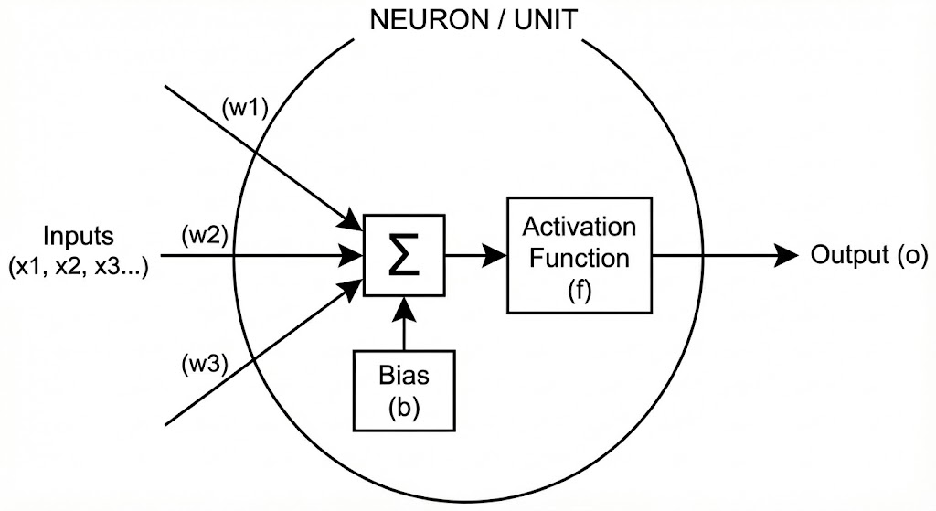Figure 1: Neuron with multiple inputs $x$, output $o$, bias $b$, and activation function $f$.

Single Layer (width n, depth 1)

In order to produce multiple outputs, we must add multiple neurons in parallel (Figure 2).

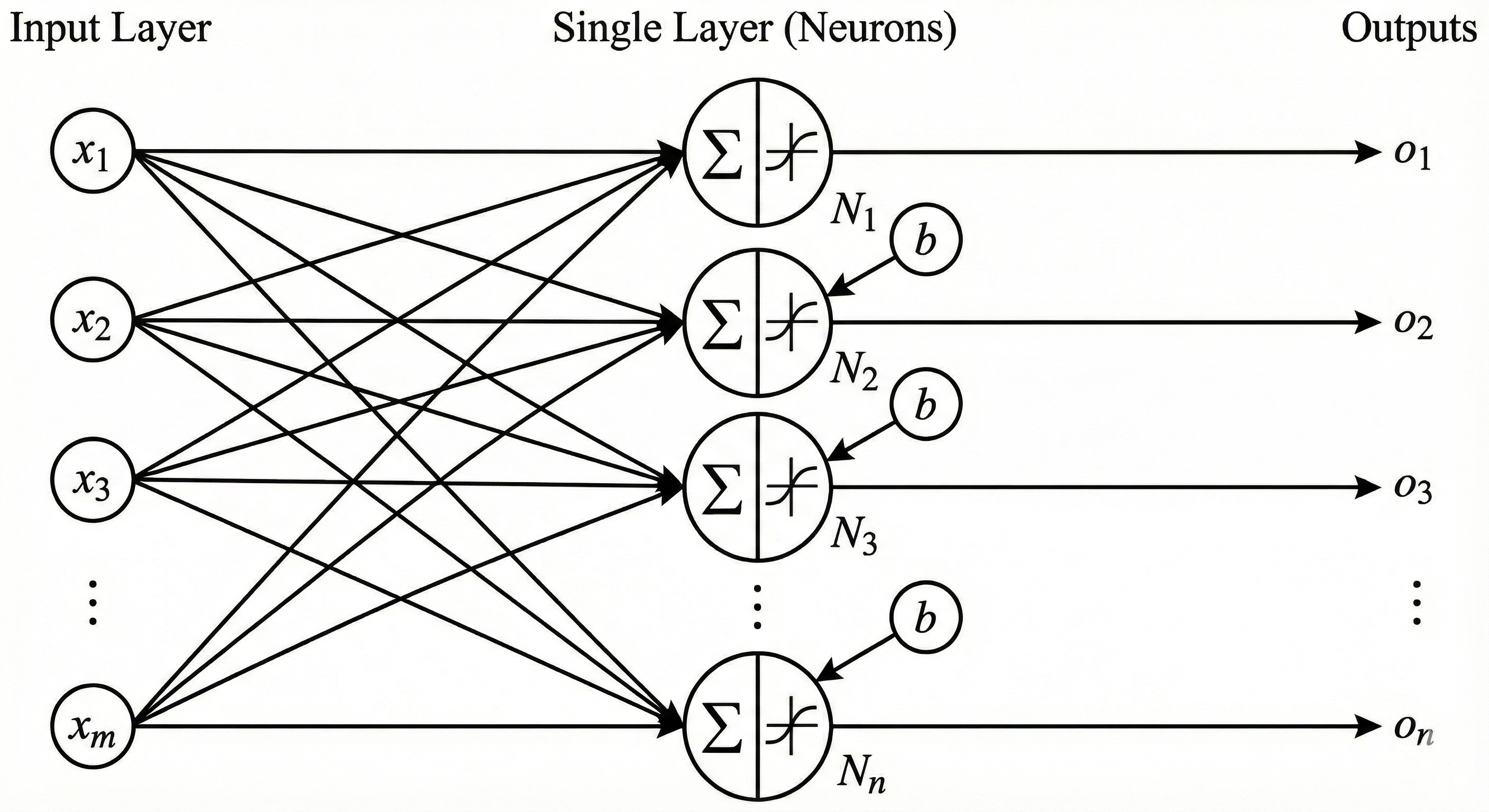Figure 2: Single layer of neurons with inputs $x$, multiple outputs $o$, bias $b$, and activation function $f$.

The only difference in mathematical formulation from the single-neuron case is the addition of an extra index accounting for each neuron. Hence, the set of weights can be organized into a matrix with entries $w_{\alpha i}$ for $i \in {1, \dots, m}$ and $\alpha \in {1, \dots, n}$. The generalized formulation becomes:

\[o_\alpha = f (w_{\alpha i} x_i + b_\alpha),\]

where $f$ is applied element-wise for each index $\alpha$.

Multiple Layers (width (p, n), depth 2)

Lastly, neural networks often consist of multiple layers, not just one. In this section, we illustrate how two layers of neurons may be connected (Figure 3).

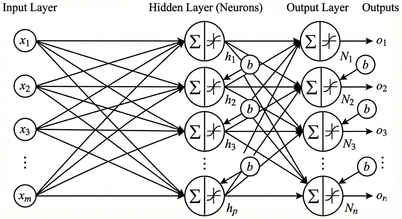Figure 3: Multiple layers of neurons with inputs $x$, multiple outputs $o$, bias $b$, and activation function $f$.

Assuming that the first layer takes inputs $x_1, \dots, x_m$ and that there are $p$ neurons in the second layer, the first layer can be described as a function $F_1: \mathbb{R}^m \to \mathbb{R}^p, \; x \mapsto o$.

The second layer then has $p$ inputs and $n$ outputs; hence, it can be described as a function $F_2: \mathbb{R}^p \to \mathbb{R}^n, \; x \mapsto o$. Together, these layers form a neural network via function composition:

\[F_\theta = F_2 \circ F_1 : \mathbb{R}^m \to \mathbb{R}^n.\]

In particular, we have

\[o_\beta = F_2 ( f (w_{\alpha i} x_i + b_\alpha)) = f ( h_{\beta \alpha} f(w_{\alpha i} x_i + b_\alpha) + b_\beta).\]

In the equation above, weights $w_{\alpha i}$ act as a transformation from $\mathbb{R}^m$ to $\mathbb{R}^p$. Similarly, weights $h_{\beta \alpha}$ transform intermediate inputs from $\mathbb{R}^p$ to $\mathbb{R}^n$. The above expression can be generalized to a neural network of arbitrary depth.

The set of parameters $\theta$

The set of all parameters of the neural network includes all the weights in the first layer $w_{\alpha i}$ and the second layer $h_{\beta \alpha}$, together with biases in both layers $b_\alpha , b_\beta$. In general, biases and weights are initialized randomly. However, weights are adjusted during training via gradient descent.

Conclusion

In this article, I described the architecture of a neural network. First, I explained how a single neuron transforms inputs into outputs. Then the concept was generalized to a single layer and finally to multiple layers. However, there are still some concepts left to explore. What is this mysterious activation function $f$? How does gradient descent work? And ultimately, how can the performance of a neural network be evaluated?